On this date I was invited by Alberto Chiarini to deliver a seminar for the cycle “Padova Seminars in Probability and Finance”, titled On the Concave One-Dimensional Random Assignment Problem: Kantorovich Meets Young. I thank the audience for many interesting remarks and later discussions, which added great value to the visit.
In this blog post, I’ll slightly expand the abstract of the seminar. Slides are available here (.pdf), and the main reference is this arXiv preprint, jointly with M. Goldman.
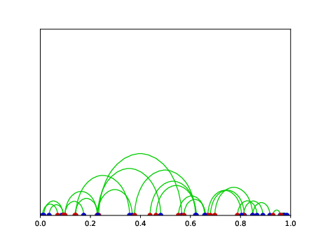
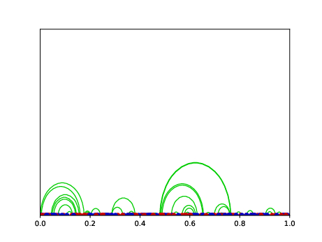
The seminar revolved around the optimal assignment problem (also known as bipartite matching problem) between \(n\) source points and \(n\) target points on the real line. What makes this problem interesting is the assignment cost, which is defined as a concave power of the distance between the points, i.e., \(|x-y|^p\), where \(0 < p < 1\).

The convex case (\(p > 1\)) has been extensively studied, and it is well-known that the solution remains constant regardless of the value of \(p\). However, in the concave case, the situation is entirely different, and the solution may vary with \(p\) and exhibit intriguing long-range connections, making it a more suitable model for real-life scenarios, and it has been proposed as a toy model for certain phenomena in economics and biology.
Taking the problem a step further, the seminar delved into the random version of the concave assignment problem. Here, the source and target points are treated as samples of independently and identically distributed (i.i.d.) random variables. The objective is to explore the typical properties of the assignment as the sample size \(n\) increases.
Barthe and Bordenave made significant progress in 2011 (.pdf) by proving asymptotic upper and lower bounds for the range \(0 < p < 1/2\), which they conjectured to be sharp. However, the full range of the problem remained elusive until Bobkov and Ledoux made more recently a groundbreaking contribution (.pdf) by leveraging optimal transport and Fourier-analytic tools: they determined explicit upper bounds for the average assignment cost in the entire range \(0 < p < 1\). This naturally led to the conjecture that a “phase transition” in the rates occurs precisely at \(p = 1/2\).
We report in our seminar that we are able to settle affirmatively both conjectures, thus resolving most of the questions surrounding the concave one-dimensional random assignment problem. This was made possible by a combination of techniques, but in particular through the development of a novel mathematical tool, which may have independent applications and is based on a formulation of the optimal transport (Kantorovich) problem using Young integration theory, where instead of transporting two different probability measures on the line, we replace them by the weak derivative of a function with finite \(q\)-variation.
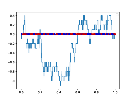
This problem can be thus correctly formulated to the Brownian bridge which provides the correct approximation of the limit between the empirical measures associated to the \(n\) source and \(n\) target points in the large \(n\) limit. Indeed, the Brownian bridge emerges by considering the difference between the empirical cumulative distribution functions of the two points, i.e., by setting a random walk that makes one step upwards every time a red point is met, and similarly but downwards for each blue point. The size of the steps must be scaled by a factor \(\approx 1/\sqrt{n}\), to have a non-trivial limit.