import numpy as np
import matplotlib.pyplot as plt
from scipy.optimize import linear_sum_assignmentToday I delivered a seminar in of the SMAQ series, in L’Aquila, hosted at the Gran Sasso Science Institute (GSSI), titled Analyzing Asymptotics of Stochastic Processes through Optimal Transport. Slides are available here for download and here is the recording of the talk.
I focused on some of the recent results obtained in the joint work with M. Mariani (arXiv:2307.10325), where we obtain upper bounds for the Wasserstein distance between the occupation measure of Brownian motion and Lebesgue measure on the flat torus.
What I believe is one of the most fascinating feature of the work, a part the fact that we conjecture our bounds to be sharp, is that we connect for the first times ideas and tools from two different mathematical areas, i.e., random bipartite matching and brownian interlacement theory. Usually these links yield new developments and I already expect extensions worth investigating (see also the last slide).
I would like to express my gratitude to the organizers, in particular Serena Cenatiempo, Nicoletta Cancrini, Alessia Nota and Davide Gabrielli for their warm hospitality.
I add below some simple Python code I used for the simulations contained in the slides.
The Brownian path is approximated as a random walk with Gaussian steps.
# The number of steps will be N^2
n = 30
N = n**2

# The stepsize is  set to be sqrt(T)/n, T being the time parameter

T=1
stepSize = T**(1/2)/n

walkSteps = np.random.normal(size=(N,2))
randomWalk = (np.cumsum(walkSteps, axis=0)*stepSize)%1
Next, we also create a uniform grid with \(N=n^2\) points.
x = np.linspace(0, 1, num=n)
y = np.linspace(0, 1, num=n)
xv, yv = np.meshgrid(x,y)
xv.resize(N)
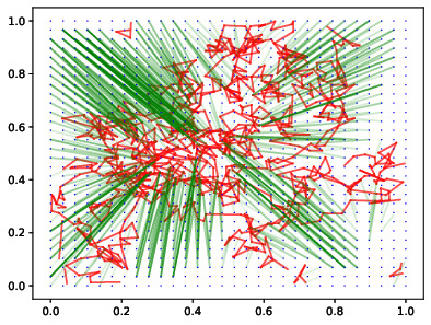
yv.resize(N)Then, we plot the grid (in blue) and the path (linearly interpolated, in red).
fig, ax = plt.subplots()

plt.plot(xv, yv, ",",  c ='blue')

# we only connect the steps that are closer than 1/2, remember that we are on the torus

for i in range(N-1):
   if np.linalg.norm(randomWalk[i]-randomWalk[i+1])<1/2:
        plt.plot( randomWalk[[i,i+1],0], randomWalk[[i,i+1], 1], c='red')

plt.show()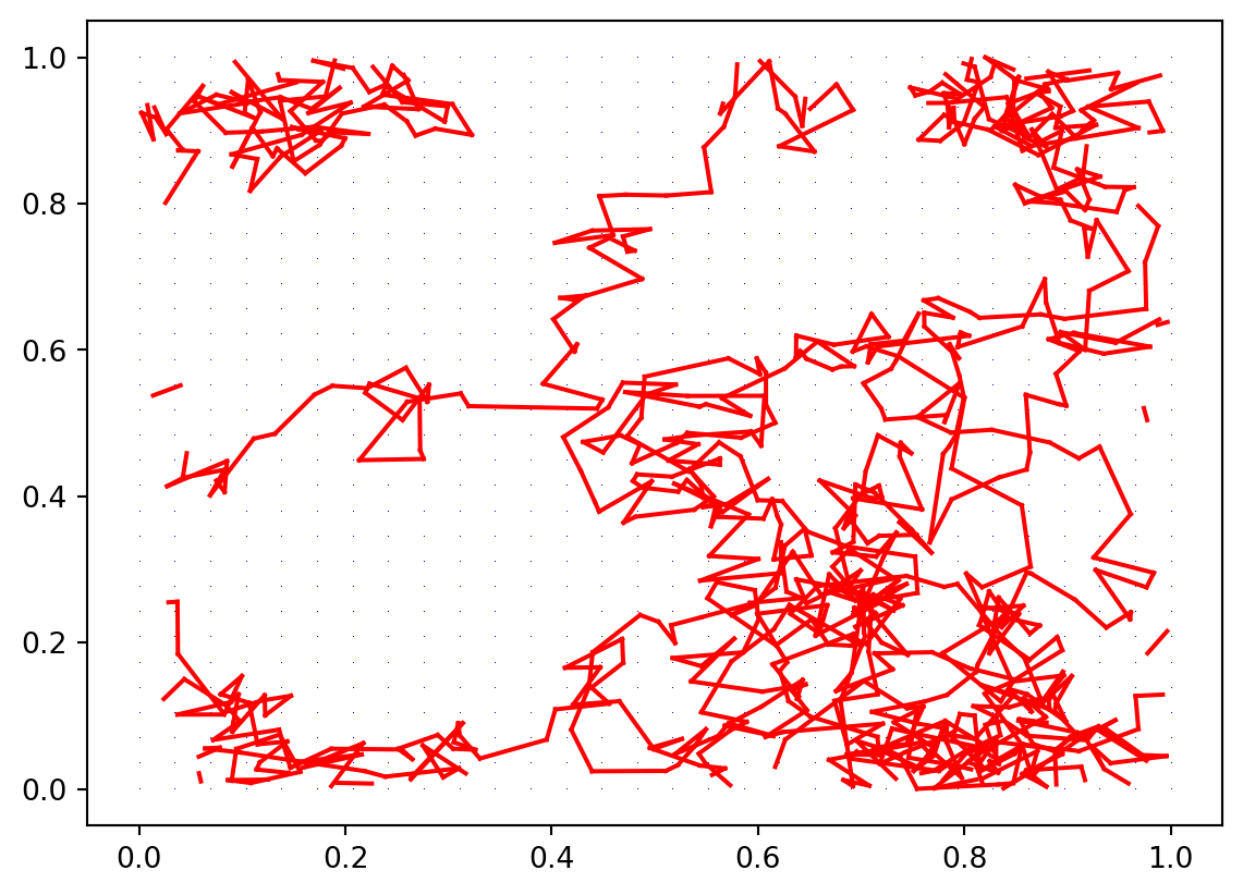
Next, we define the unit transport cost given by the distance on the flat torus.
def cost(a,b, p=1):
    return  (min(np.abs(a[0]-b[0]), 1-np.abs(a[0]-b[0]))**2 + min(np.abs(a[1]-b[1]), 1-np.abs(a[1]-b[1]))**2)**(p/2)
We use it to build a cost matrix containing all the distances between red and blue points.
costMatrix = np.zeros( (N, N))
for i in range(N):
    for j in range(N):
            costMatrix[i,j] = cost( randomWalk[i],  [xv[j], yv[j]])
We solve the bipartite matching problem using Munkres algorithm and plot the solution (with a little tweak one can also re-plot the red path and blue points).
x_sol, y_sol = linear_sum_assignment(costMatrix)

fig, ax = plt.subplots()


for i in range(N):
    matchingLength = np.linalg.norm( randomWalk[x_sol[i]]- [xv[y_sol[i]], yv[y_sol[i]]])
    if matchingLength <1/2:
         plt.plot( [randomWalk[x_sol[i], 0], xv[y_sol[i]]], [randomWalk[x_sol[i], 1], yv[y_sol[i]]], alpha=2*matchingLength, c='green')

plt.show()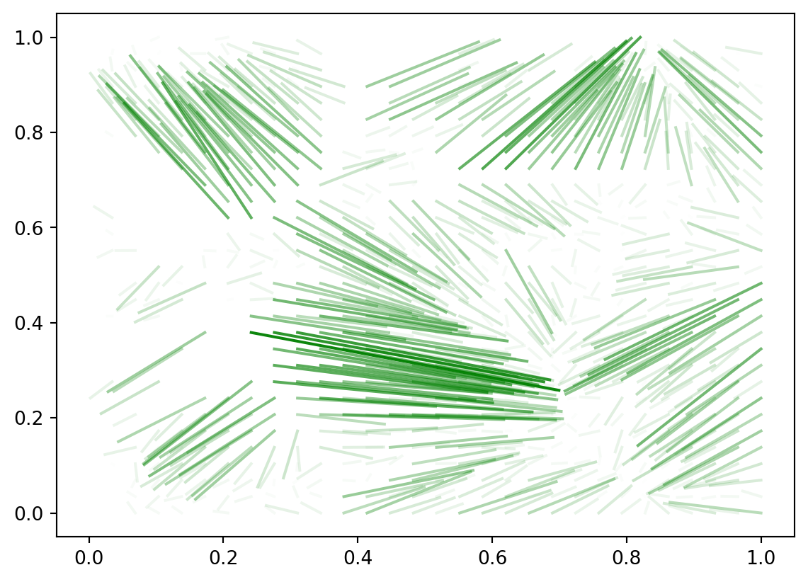
I am pretty sure that faster and possibly better-looking simulations can be performed using ad-hoc modules such as POT, in particular by computing directly the semi-discrete optimal transport between the random walk points and the uniform measure.