Interframe Gap Shrinkage

We finish the evaluation of the network shown in Figure 7.3 by calculating the worst-case interframe gap shrinkage for that network. This is done by evaluating the same worst-case path that we used in the path delay calculations. However, for the purposes of calculating gap shrinkage we only evaluate the transmitting and mid-segments.

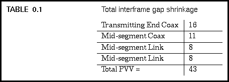
Once again we start by applying the network model to the worst-case path. For interframe gap shrinkage the transmitting segment should be assigned the end segment in the worst-case path that has the largest shrinkage value. As shown in Table 7.2, the coax segment has the largest value, so we will assign the 10BASE2 segment to the role of transmitting end segment. The mid segments consist of one coax and two link segments. That leaves the 10BASE-T receive end segment which is simply ignored. The totals are:

As you can see, the total path variability value for our sample network equals 43. This is less than the 49 bit time maximum allowed in the standard, which means that this network meets the requirements for interframe gap shrinkage.

Quick Reference Guide to 10-Mbps Multi-Segment Configuration - 09 SEP 95

[Next] [Previous] [Up] [Top] [Copyright] [Books About Ethernet]

Generated with CERN WebMaker